Linear regression using sklearn (scikit-learn) in Python

What is linear regression?

Linear regression is a simple and useful mathematical method used in the data analysis and machine learning. Its goal is to find linear relationship between dependent variable and one or more independent variables. When the number of independent variables is one, then it’s called univariate or simple linear regression. In the case of more than one independent variable, it is known as multivariate or just multiple linear regression. The dependent variable is also called the output or response. The independent variables are called independent features, regressors, inputs, or predictors.

Applications of linear regression

Linear regression is widely used in various fields, such as economics, social sciences, natural sciences, engineering, etc. The importance of this method is demonstrated by the fact that we can find dozens of books devoted exclusively to this method. It appears in almost every econometrics textbook¹. It is also common in scientific articles. Scientists often try to find relationships between variables, thanks to which they can understand the problem under study . We can find interesting examples of the use of linear regression in scientific research. The book Linear Regression Analysis: Theory and Computing² describes an experiment that examined the effect of cigarette smoking on mortality. Another interesting scientific research is a study _³ in which this method was used to determine the author’s age based on the texts.

How linear regression is calculated?

Finding a linear relationship involves determining the coefficients of a straight line. The least squares method can be used for this purpose. It is based on minimizing the sum of the squares of the the residuals (SSE – Sum of Squared Error), defined as:

$SSE=\sum_{i=1}^{n}[y_i-\bar{y}_i]^2$

where:

y_i – value of y at point i

$\bar{y}_i- \text{predicted value of } \textit{y} \text{ at point } \textit{i}$

The function SSE is minimized to find the best fit line.

The condition for SSE to be a minimum is:

$\frac{\partial SSE}{\partial a_i}$

for i = 1,…,n

Python libraries used in linear regression

In Python, we have two main libraries that can be used for linear regression: scikit-learn (also written sklearn – they are the same thing) and statsmodels. The latter is much more extensive and we will not need to use its functionality. The scikit-learn library includes all the key functions for most analyses. Performing linear regression in Python using the scikitlearn library is very simple. In addition to this library, we will also use:

numpy – a library for calculations, especially on matrices,
matplotlib – a library for creating plots,
pandas – a library for data science.

Code for simple linear regression in Python

This tutorial shows how to use most popular library for scientific computing in Python – scikit-learn. We will consider two examples: simple and multiple linear regression and calculate coefficients describing the quality of fit.

Step 1. Import required libraries

import numpy as np
import matplotlib.pyplot as plt
from sklearn.linear_model import LinearRegression
from sklearn.metrics import r2_score

Step 2. Import the dataset

Typically, we will import the data from a file. In this example, we will use data generated using the numpy library. Vector X will contain random values between 0 and 1, while y will be the values computed from the line equation to which a random “error” will be added.

np.random.seed(0)
X = np.random.rand(100, 1)  # Independent variable
y = 3 * X + 2 + np.random.randn(100, 1)/10  # Dependent variable + "error"

Step 3. Create the linear regression model

The LinearRegression() method was previously imported from the sklearn library. To fit a line to the X, y data, we call the fit() method.

# Linear regression model creation and fitting
model = LinearRegression()
model.fit(X, y)

Step 4. Evaluate the regression

We will use the R squared coefficient to evaluate the fit of the straight line. We know from the theory that its value should be as close as possible to one, which proves that the line fits the data well. If the value is much less than one (“significantly” depends on the particular problem), then there is no linear relationship between the data X and y. To determine R squared, we first calculate the y values predicted by the created linear model (the predict method) for the existing X values. Then we use the obtained values to call the r2score method.

# Values predicted by the model
y_pred = model.predict(X)

# Calculation of R squared
r2 = r2_score(y, y_pred)

print("R squared:", r2)

In regression there are also other metrics used to assess the quality of fit. These are three coefficients: mean absolute error, mean square error and root mean square error. The sklearn library has methods to determine their values, as shown below.

from sklearn import metrics
print('Mean Absolute Error:', metrics.mean_absolute_error(y, y_pred))  
print('Mean Squared Error:', metrics.mean_squared_error(y, y_pred))  
print('Root Mean Squared Error:', np.sqrt(metrics.mean_squared_error(y, y_pred)))

The parameters of the line a*x + b are obtained from the attributes of the model object. coef_ is parameter a (slope) and intercept_ is b (intercept).

# Coefficient a in the equation y = a*x + b
a = model.coef_
print("Coefficient a:", a)

# Coefficient b in the equation y = a*x + b
b = model.intercept_
print("Coefficient b:", b)

Step 5. Visualize the results

To visualize the data and results we will use the Matplotlib library. We will create a scatter plot. The xlabel and ylabel methods are used to describe the axes, and the legend() methods are used to create a legend on which labels previously assigned will be displayed. We display the graph using show().

plt.scatter(X, y, color='blue', label='Data')
plt.plot(X, y_pred, color='red', linewidth=2, label='Linear regression')
plt.xlabel('X')
plt.ylabel('y')
plt.legend()
plt.show()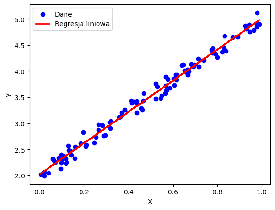

Code for multiple linear regression in Python

Multiple linear regression concerns a problem in which there are multiple independent variables (also called features). In this example we will use a csv file containing data about houses prices.

Step 1. Import libraries

import numpy as np
import pandas as pd
from sklearn.linear_model import LinearRegression
from sklearn.model_selection import train_test_split

Here we use pandas library to manage data, which is one of most popular libraries used in data science.

Step 2. Read data from file to dataframe

#  Load data set 
df  = pd.read_csv('houses.csv', sep=';')

# show first five rows
df.head()

	size	years_old	bedrooms	price
0	2500	20	3	770000
1	3100	16	4	950000
2	3300	3	18	1010300
3	4000	4	10	1220000
4	3200	6	6	977000

We see that there are three features: size, years_old and bedrooms. Price is the output variable (dependent variable).

Step 3. Choose the features and output

# X = df.drop(columns=['price']) # Independent variables
X = df.drop(columns=['price'])
y = df['price']  # Dependent variable

Step 4. Split the data into training and testing sets.

X_train, X_test, y_train, y_test = train_test_split(X, y, test_size=0.2, random_state=42)

This is an important step, in which data is divided into two sets. The training set will be used for finding the coefficients of the model. The test set will be used to evaluate the goodness of fit.

Step 5. Train the model

# Create a Linear Regression model
model = LinearRegression()

# Fit the model to the training data
model.fit(X_train, y_train)

Step 6. Evaluate the model

from sklearn.metrics import mean_squared_error, r2_score

# Predict on the test set
y_pred = model.predict(X_test)

mse = mean_squared_error(y_test, y_pred)
r2 = r2_score(y_test, y_pred)

print(f"Mean Squared Error: {mse:.2e}")
print(f"R-squared: {r2:.2}")

# Access the coefficients
intercept = model.intercept_
coefficients = model.coef_ 

# Round the intercept
rounded_intercept = round(intercept, 2)

# Round all coefficients
rounded_coefficients = [round(coef, 2) for coef in coefficients]

print("Intercept:", rounded_intercept)
print("Coefficients:", rounded_coefficients)

Output:

Mean Squared Error: 2.27e+10
R-squared: 0.81
Intercept: -359.84
Coefficients: [302.48, 604.63, 565.46]

The code above calculates the R-squared coefficient, MSE and also prints regression coefficients.

Summary

Linear regression is an important method used in engineering, data science and machine learning. From this article you learned what linear regression is and how to write a program that creates a linear regression model in Python. In particular, you learned how to:

use the scikit-learn library to create a simple linear regression model and multiple regression,
determine the coefficients of linear relationship and the coefficient of determination R²,
draw a graph with the data and the regression line.

References