Dynamical simulation of a heating tank (part 2)

This is a part of the lecture notes in process control.

Model of a heating tank

The model of a mixed tank heated up by water steam consists of two equations: one for the heating phase and one for the cooling phase:

– heating phase:

(1) $T(t)=\frac{{{T}_{f}}+\tau Q{{T}_{q}}}{1+\tau Q}+\left( {{T}_{low}}-\frac{{{T}_{f}}+\tau Q{{T}_{q}}}{1+\tau Q} \right)\cdot \exp \left( -\frac{1+\tau Q}{(1+\varepsilon )\tau }t \right)$

with the initial condition:

(2) $T(0)={{T}_{low}}$

– cooling phase:

$T(t)={{T}_{f}}+\left( {{T}_{high}}-{{T}_{f}} \right)\cdot \exp \left( -\frac{1}{(1+\varepsilon )\tau }t \right)$

with the initial condition:

(4) $T(0)={{T}_{high}}$

Analysis of a dynamical system

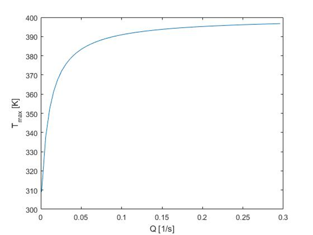
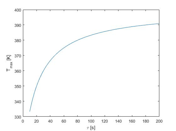
Let’s look at the solution obtained. We can calculate the maximum temperature which can be obtained in the system, assuming the heating phase lasts sufficiently long. It can be done by finding the limit:

(5) $\underset{t\to \infty }{\mathop{\lim }}\,T(t)=\frac{{{T}_{f}}+\tau Q{{T}_{q}}}{1+\tau Q}$

Based on this Eq. we can state that there are several ways to obtain higher temperature. First of all, one method is to increase temperature of water steam, T_q. Other possibilities are based on increasing parameter Q (reflecting heat transfer rate) or τ (residence time of the liquid). The influence of these parameters on the maximum possible temperature is illustrated in Fig. 1 and Fig. 2.

Fig. 1. Influence of parameter Q on the maximum possible temperature

Fig. 2. Influence of parameter τ on the maximum possible temperature

We can also calculate the temperature which will be obtained in the system when the cooling phase lasts sufficiently long:

(6) $\underset{t\to \infty }{\mathop{\lim }}\,T(t)={{T}_{f}}$

The above equation simply states that after sufficiently long time of the cooling phase, the liquid flowing through the tank will finally get the temperature of the inlet stream.

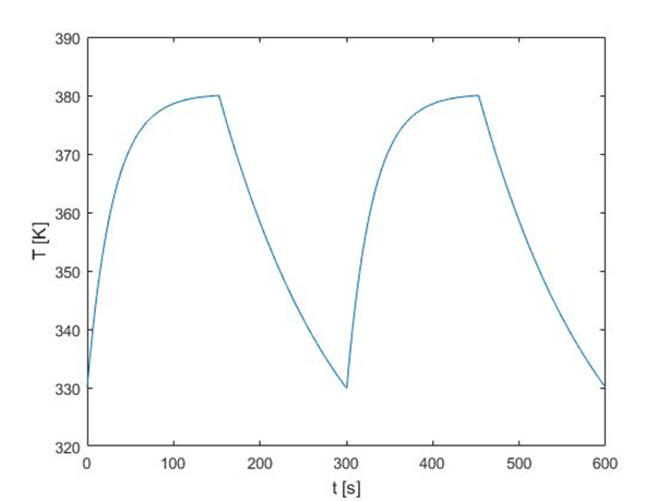
Let’s simulate the dynamic operation of this object. To this purpose it is necessary to choose values of parameters. We will take the following:

T_f = 300 K, T_q = 400 K, τ = 100 s, Q = 0.04075 1/s, ε = 0.5, T_low= 330 K, T_high= 380 K, T(0)= 330 K.

The solution is given by explicit expressions, so no additional transformations are required. We will use Eq. () for heating phase and Eq. () and cooling phase following one after another, when the switching temperature (T_max or T_low) are crossed. The Matlab m-file attached to this lecture plots the relationship T(t), which is presented in Fig. 3.