What is PID control?
Proportional-integral-derivative (PID) controllers have been used in manufacturing industry since the 1940s. PID control is similar to proportional control, but with the addition of integral and derivative components. The integral feature eliminates the offset while the derivative element provides a fast response.
Let’s start with a bit of theory. The following equation is used by PID controller to compute the output value u(t):
![\[u={{K}_{p}}e(t)+{{K}_{i}}\int\limits_{0}^{t}{e(\tau )d\tau }+{{K}_{d}}\frac{de(t)}{dt}\]](https://softinery.com/wp-content/ql-cache/quicklatex.com-ad30e6ff874f517880ff5057bb2d8ac6_l3.png "Rendered by QuickLaTeX.com")
Kp, Ki and Kd denote the coefficients for the proportional, integral, and derivative gains respectively; e denotes error and t – time.
In this tutorial you will learn how to use Python programming language to implement PID controller.
PID controller – Example of application
The system
Let’s consider a tank used to continuously heat up the liquid stream flowing through this tank with heating jacket shown in the figure. We can use the PID controller to obtain temperature set. We will use a simple mathematical model of this system (check more detailed description in this lecture).
![\[\frac{dT}{dt}=\frac{1}{1+\varepsilon }\left[ \frac{1}{\tau }({{T}_{f}}-T)+Q({{T}_{q}}-T) \right]\]](https://softinery.com/wp-content/ql-cache/quicklatex.com-e21839e12a4d8e53aec331d699c9d9ee_l3.png "Rendered by QuickLaTeX.com")
![\[\varepsilon =\frac{{{m}_{s}}{{c}_{s}}}{V\rho {{c}_{p}}},\ Q=\frac{{{A}_{q}}{{k}_{q}}}{V\rho {{c}_{p}}},\ \tau =\frac{V}{{{F}_{V}}}\]](https://softinery.com/wp-content/ql-cache/quicklatex.com-9ad53284cf2580f3df736086c5bce4dd_l3.png "Rendered by QuickLaTeX.com")

Python code of a system with PID control
Let’s start writing the program with importing necessary python libraries.
import numpy as np
import matplotlib.pyplot as plt
from scipy.integrate import odeint
import numpy as np
import matplotlib.pyplot as plt
We will need several global variables as the calculations require the history of the object.
time = 0
integral = 0
time_prev = -1e-6
e_prev = 0
The function below calculates the value of the manipulated variable (MV) based on the measured value (in example it is the temperature of the liquid) and setpoint value (temperature we want to obtain). The function also accepts parameters of the controller.
def PID(Kp, Ki, Kd, setpoint, measurement):
    global time, integral, time_prev, e_prev

    # Value of offset - when the error is equal zero
    offset = 320

    # PID calculations
    e = setpoint - measurement

    P = Kp*e
    integral = integral + Ki*e*(time - time_prev)
    D = Kd*(e - e_prev)/(time - time_prev)

    # calculate manipulated variable - MV
    MV = offset + P + integral + D

    # update stored data for next iteration
    e_prev = e
    time_prev = time
    return MV
Next, we create a function defining the system.
def system(t, temp, Tq):
    epsilon = 1
    tau = 4
    Tf = 300
    Q = 2
    dTdt = 1/(tau*(1+epsilon)) * (Tf-temp) + Q/(1+epsilon)*(Tq-temp)
    return dTdt
Let’s see the results for the system without the automatic control. We obtain them by solving the differential equations shown before.
tspan = np.linspace(0,10,50)
Tq = 320,
sol = odeint(system,300, tspan, args=Tq, tfirst=True)
plt.xlabel('Time')
plt.ylabel('Temperature')
plt.plot(tspan,sol)
We see that the temperature in the tank is equal 300 K at the initial time and it rises to about 317.5 steadily. Now, we will make a simulation of the tank with automatic control. Let’s say that we want to reach the temperature of 310 K. This is our setpoint. The controller constants are set arbitrarily – they can be adjusted to get a better control. However, it is out of the scope of this tutorial. Temperature of steam was chosen as a manipulated variable (Tq). You can see that its value is calculated in every step of simulation with the use of previously written PID function.
# number of steps
n = 250

time_prev = 0
y0 = 300
deltat = 0.1
y_sol = [y0]
t_sol = [time_prev]

# Tq is chosen as a manipulated variable
Tq = 320,

q_sol = [Tq[0]]
setpoint = 310
integral = 0
for i in range(1, n):
    time = i * deltat
    tspan = np.linspace(time_prev, time, 10)
    Tq = PID(0.6, 0.2, 0.1, setpoint, y_sol[-1]),
    yi = odeint(system,y_sol[-1], tspan, args = Tq, tfirst=True)
    t_sol.append(time)
    y_sol.append(yi[-1][0])
    q_sol.append(Tq[0])
    time_prev = time

plt.plot(t_sol, y_sol)
plt.xlabel('Time')
plt.ylabel('Temperature')
You can see that the controller makes the temperature tend to the desired value.
Download Jupiter notebook file with PID implementation
Download from Github.
Read related content
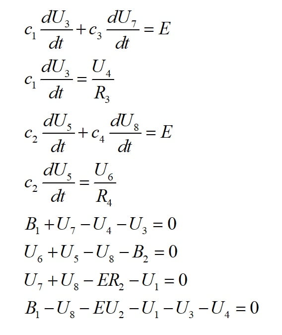
How to solve system of DAEs in Python
Lecture notes in process control

Need process simulation consultant? Contact us
We are here to help. Contact us by phone, email or via our social media channels.
Nice