How to solve differential equations in Python?
This tutorial shows how to use Python for solving differential equations which are one of the most important problems in engineering. We will discuss several examples, as the whole subject is extremely wide and requires a lot of theory. I will use Scipy library which is very simple in use.
Differential equations – definition
Differential equation is is an equation with one or more derivatives of a function. While differential equations are commonly divided into ordinary (ODE) and partial ones (PDE), they can be further described by order, linearity, and degree (Fig. 1).

Applications and examples of differential equations
Differential equations are very common, as they are perfect for description of real world. Here, we have few examples in different areas of engineering and science:
- biochemical engineering, for example growth of microorganisms
(1) ![]()
- process engineering, for example heat transfer
(2) ![]()
- mechanical engineering, for example spring-mass system
(3) ![]()
Solve first-order ordinary differential equation with SciPy
A first-order differential equation (ODE) is an equation of the form F(t,y,y′)=0. Some of them can be solved analytically, without using a computer. Some of them require numerical solution, using proper computer algorithm. Numerical solution does not provide explicit function, just tabular data. In many cases it is sufficient for further analysis of the problem. The odeint method is an example of numerical solvers. We will use it for the following problem:
(4) ![]()
![]()
First, let’s import necessary libraries. We will use odeint from scipy to solve the equation. We will also use numpy and matplotlib.
from scipy.integrate import odeint
import numpy as np
import matplotlib.pyplot as plt
Next, let’s write the function defining the equation. As a rule, we leave the derivative on the left-hand-side of the equation. The python function calculates the expression on the right-hand-side.
def returns_dydt(y,t):
    dydt = -y * t + 13
    return dydt
We need one initial value y0, as we deal with first-order differential equation. The array t consists of time values for which the solution will be obtained. The function odeint from scipy calculates the result of the ODE for given function, initial value and time array, as below.
# y value at time 0
y0 = 0
# values of time - from 0 to 5.
t = np.linspace(0,5,10)
# solving ODE
y_result = odeint(returns_dydt, y0, t)
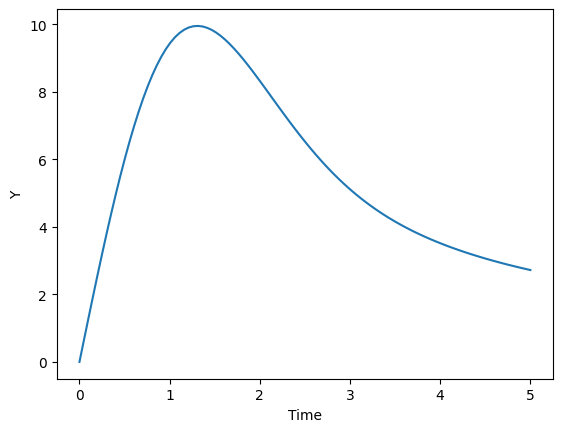
Now we can plot the result. To do that we need two arrays: t and y_result.
# plot results
plt.plot(t,y_result)
plt.xlabel("Time")
plt.ylabel("Y")
plt.show()
Solve system of ordinary differentia equations (ODEs)
Let’s consider the following problem:
(5) 
![]()
The solution is similar to a single ODE. The main difference is in the function defining right-hand-sides of the system. Now, Y consists of two values y1 and y2, and the function returns two expressions, according to equations in the system.
def dYdx(Y, x):
    y1, y2 = Y
    return [2 * y2 + x,
           2 * y1 + 3 * np.sin(x)]
After defining initial conditions, we will use odeint function. It accepts three arguments: the function, tuple with initial conditions and array of independent variable values.
# y1 and y2 values at time 0
y1_0 = 0
y2_0 = 1

# Vector of indipendent variable
x = np.linspace(0, 1, 50)
# Solution
sol = odeint(dYdx, (y1_0, y2_0), x)
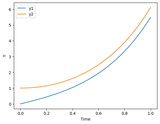
The solution consists of two functions, y1(x) and y2(x). The sol matrix store them in separate columns. We can use them to plot the results, as below:
# Unpack variables
y1 = sol[:,0]
y2 = sol[:,1]

# Plot
plt.plot(x, y1, label='y1')
plt.plot(x,y2, label='y2')
plt.xlabel("Time")
plt.ylabel("Y")
plt.legend(loc='upper left')
plt.show()
Summary
In this tutorial we presented how to solve ordinary differential equations and systems of ordinary differential equations in Python. Differential equations are often used in engineering and science for the description of real objects, including dynamic systems. You can find examples of application of the presented methods in our blog, for the simulation of batch bioreactor, plug-flow reactor or a system with PID control.
