A differential-algebraic equation (DAE) is an equation involving an unknown function and its derivatives. A (first order) DAE in its most general form is given by:

How to a solve system of differential-algebraic equations in Python

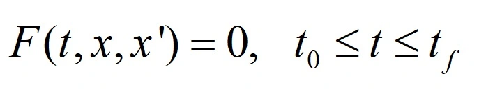
where x = x(t) , the unknown function, and F=F(t, u, v) have N components, denoted by x_iand F_i, i = 1,2,…,N, respectively.

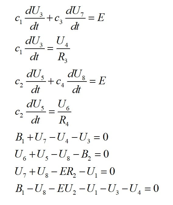
Example

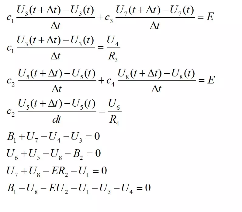
Let’s consider the following problem:

System of differential-algebraic equations

There are several libraries which can be used for solving such problems, but there are sometimes problems with installation. This time, I will show how to solve such problem using fsolve from SciPy.

The method involves discretization of time derivatives. Instead of dU_i/dt we use ΔU_i/Δt_i:

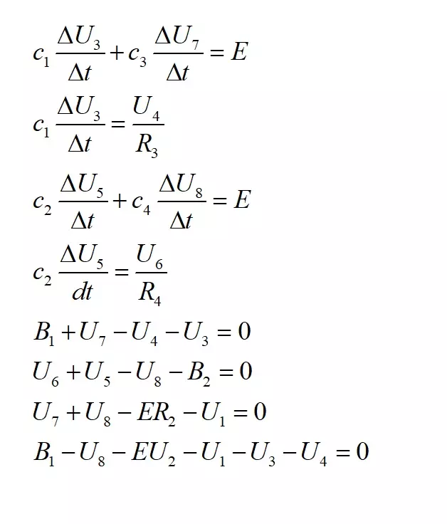
Value of ΔU_i is equal to difference between two consecutive time values. Then we get:

Discretization of DAE - finite differences

This way, the system of differential-algebraic equations was transformed to a system of algebraic equations. Now, we need to move non-zero elements to left-hand-side of the equation, as follows:

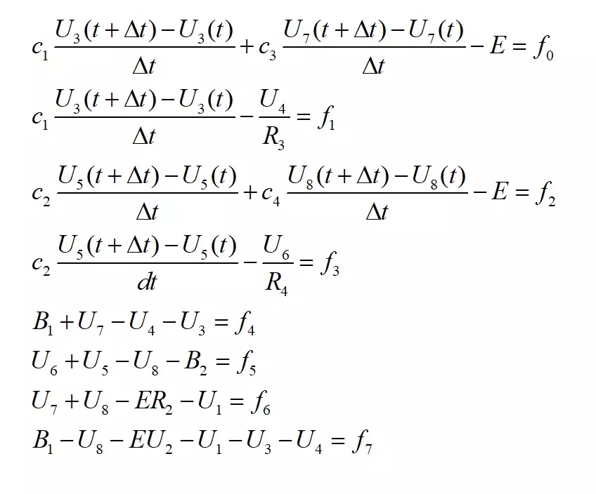
Finally, at every time step we need to solve system of algebraic equations f₀, f₁,…f₇.

Solution of a system of differential-algebraic equations

The necessary imports:

import numpy as np
from scipy.optimize import fsolve
import matplotlib.pyplot as plt

First, we will define function describing the algebraic equations:

def dae_eqs(U, *args):

    # U denotes vector of variables at time t + time_step. U(0) means U1, U(1) is U2 and so on.

    # *args contains Ut and time_step
        # Ut denotes vector of variables at time t.
        # value of time step is necessary for calculating discretized derivatives.

    # Unpack arguments
    Ut, time_step = args
    # set some arbitray values of parameters
    c1 = 1.0
    c2 = 2.0
    c3 = 3.0
    c4 = 4.0
    R2 = 2.0
    R3 = 3.0
    R4 = 4.0
    B1 = 1.0
    B2 = 2.0
    E = 5.0

    # Let's assign values of U array to U1, U2, ... for ease.
    U1 = U[0]
    U2 = U[1]
    U3 = U[2]
    U4 = U[3]
    U5 = U[4]
    U6 = U[5]
    U7 = U[6]
    U8 = U[7]
    # The same for array Ut.
    Ut1 = Ut[0]
    Ut2 = Ut[1]
    Ut3 = Ut[2]
    Ut4 = Ut[3]
    Ut5 = Ut[4]
    Ut6 = Ut[5]
    Ut7 = Ut[6]
    Ut8 = Ut[7]

    # Derivatives of U valuses. Some of them are not used, but let's leave them for consistency.
    U1_deriv = (U1-Ut1)/time_step
    U2_deriv = (U2-Ut2)/time_step
    U3_deriv = (U3-Ut3)/time_step
    U4_deriv = (U4-Ut4)/time_step 
    U5_deriv = (U5-Ut5)/time_step
    U6_deriv = (U6-Ut6)/time_step
    U7_deriv = (U7-Ut7)/time_step   
    U8_deriv = (U8-Ut8)/time_step   

    # calculate values of algebraic equations
    f0 = c1 * U3_deriv + c3 * U7_deriv - E
    f1 = c1 * U3_deriv - U4/R3
    f2 = c2 * U5_deriv + c4 * U8_deriv - E
    f3 = c2 * U5_deriv - U6/R4
    f4 = B1 + U7 - U4 - U3
    f5 = U6 + U5 - U8 - B2
    f6 = U7 + U8 - E*R2 - U1
    f7 = B1 - U8 - E*U2 - U1 - U3 - U4

    # Gather all fs into one array
    f = np.array([f0, f1, f2, f3, f4, f5, f6, f7])
    return f

According to the explanation in the first part of the article, the main program looks as follows:

# set initial conditions for t = 0
number_of_unknowns = 8
U = np.zeros(number_of_unknowns)

# If initial conditions are different from zero, they should be set separately, as below
U[0] = 1.0
U[1] = 1.0
U[2] = 1.0
U[3] = 1.0
U[4] = 1.0
U[5] = 1.0
U[6] = 1.0    
U[7] = 1.0   

# set time step, end_time and time
time_step = 0.1
end_time = 5
time = 0

# Initial condition must satisfy the system. Therefore it is required to find proper solution at time 0.
u_0 = fsolve(dae_eqs, U, args=(U,time_step))

# Create arrays for storing solution
time_solution = np.linspace(0, end_time, (int)(end_time/time_step)+1)
u_solution = np.zeros((time_solution.size, number_of_unknowns))
i = 0
u_solution[0] = u_0 # assign initial condition
while time < end_time - time_step:
    args = (U, time_step) # arguments for fsolve
    u_next =  fsolve(dae_eqs, U, args=args) # calculate u at time t + time_step
    U = u_next # in next iteration U is equal U from previous iteration 
    u_solution[i+1] = u_next
    time += time_step # increase time
    i += 1

We can plot some results now:

fig, ax = plt.subplots(2)
ax[0].plot(time_solution, u_solution[:,0])

ax[0].set(ylabel='U1')
ax[0].grid()

ax[1].plot(time_solution, u_solution[:,1])

ax[1].set(xlabel='time (s)', ylabel='U2')
ax[1].grid()

#Plot the solution of differential-algebraic equations
plt.show()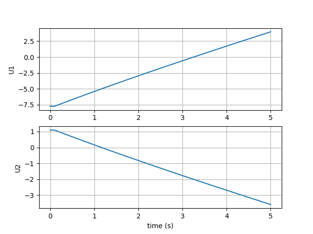

Summary

Above, we have seen how to solve differential-algebraic equations in Python. Such problems appear in many fields of engineering, including biochemical, electrical and process engineering.

The above method is not perfect. It uses the simplest discretization and it will not always work, for example, if one deals with stiff differential equations. There are several Python libraries which can be used. Some of them are listed below:

https://pypi.org/project/diffeqpy/

https://lcvmwww.epfl.ch/software/daepy/

You can lear more about DAEs on Scholarpedia.

If you want to learn more about solving engineering problems using Python, see the offer for the Course: Python in engineering and science