Shooting method - boundary value problem in Matlab and Python

What is a shooting method?

Shooting method is a numerical method used for solving boundary value problems (BVP). It is based on reducing it to an initial value problem with unknown initial condition(s) which is to be found for example by Newton’s Raphson [1]. To explain it, let’s first define a BVP. It is a system of differential equations with solution and derivative values specified at more than one point. Many engineering problems are described by two-point boundary value problem, which can be described as N coupled first-order ordinary differential equations, satisfying n₁ conditions at point x₁ and n₂ = N–n₁ conditions at point x₂. In mathematical notation in can be written as [2]:

(1) $\frac{dy_i}{dx}=g_i(x,y_1,y_2,...,,y_N) \ , \ \ \ i=1,2,...N$

At x₁ the solution satisfies:

(2) $B_{1j}(x_1,y_1,y_2,...,,y_N) \ , \ \ \ i=1,2,...n_1$

while at x₂ the solution satisfies:

(3) $B_{2k}(x_1,y_1,y_2,...,,y_N) \ , \ \ \ k=1,2,...N-n_1$

In the shooting method we assume all values of the dependent variables (y_i) at x₁, which are consistent with the boundary condition at x₁. Afterwards, we integrate the differential equations (ODEs) up to x₂. The values of dependent variables obtained at the boundary x₂ are then compared with the known boundary conditions. Based on the discrepancy, the values of y_i at at x₁ are corrected. The ODEs are then integrated once again. The whole procedure is repeated unless satisfying accuracy of the values y_i at x₂. The shooting method is illustrated in Fig. 1. We can think of this method as taking shots, which we correct each time by checking whether we hit the target.

shooting method - illustration — Fig. 1. The principle of shooting method

Shooting method in Matlab

Let’s solve the following second-order differential equation:

(4) $\frac{d^2y}{dx^2}+x \frac{dy}{dx}+2y=0$

with boundary conditions: y(0) = 1 and y(2) = 8.

We need to convert second-order differential equations into a system of first-order ones. It is done by introducing new variable:

(5) $y_2=\frac{dy}{dx}$

After differentiation:

(6) $\frac{dy_2}{dx}=\frac{d^2y}{dx^2}$

After substituting y by y₁ and introducing y₂ and dy₂/dx into Eq. (4) we get:

(7) $\frac{dy_2}{dx}+x y_2+2y_1=0$

Finally, we obtain a system of two first-order ODEs by combining the Eq. (7) and the definition (5):

(8a) $\frac{dy_1}{dx}=y_2$

(8b) $\frac{dy_2}{dx}=-x y_2-2y_1$

Please note that we present the equation in the form in which the left-hand sides contains only the derivatives of dependent variables. The boundary conditions are unchanged, that is: y₁(0) = 1 and y₁(2) = 8. In case they are specified for the derivative of y, it is necessary to transform them by introducing the new variable y₂.

In Matlab we will split the problem into three functions. The first one will define the right-hand sides of the system of ODEs.

MATLAB

function dy = rhs(x,y)
    dy = zeros(2,1);
    dy(1) = y(2);
    dy(2) = -x * y(2) - 2 * y(1);
end

The construction is rather straightforward. The parameters of the functions are the independent variable x and vector of dependent variables y. The function returns vector of derivatives dy. The next function defines the boundary condition, as below:

MATLAB

function F = bc(x)
    options = optimoptions('fsolve','TolX',1e-8,'TolFun',1e-10');
    [X,YY] = ode45(@rhs,[0 2],[1 x],options);
    s=size(YY);
    y1_right=YY(s(1),1);
    y2_right=YY(s(1),2);
    F = y1_right-8;
end

We see that the there is a parameter of the function (x). It is the unknown initial condition. It is used in ode45 solver for integration of the equations in rhs function. After integrating, we use YY matrix to find the values of dependent variables at the right end of the domain. The value of y₁ is the last element in the first column of the solution YY. The boundary condition is defined in the form: 0 = y₁(2) – 8. Such notation is required by fsolve solver which will be used to find the unknown initial condition.

The function below below uses the fsolve solver to find the unknown initial condition, defined in bc function. The value x found by the solver is afterwards used to integrate the ODEs once again to obtain the solution. The function returns two variables: vector X and matrix Y which stores the values of dependent variables y.

MATLAB

function [X,Y]=shoot_find()
    options = optimoptions('fsolve','TolX',1e-8,'TolFun',1e-6');
    x = fsolve(@bc,1e-6,options);
    [X,Y]=ode45(@rhs,[0:0.01:2],[1 x],options);
end

In the fsolve solver (line three), the value 1e-6 is used as an initial guess. The algorithm will start searching for the solution using this value. Finally, we can use the above functions (rhs, bc and shoot_find) to find the solution of the problem. To do this we run the shoot_find function and plot the result as below.

MATLAB

function shoot_method_problem_1()
    [X,Y]=shoot_find();
    plot(X,Y(:,1))
    legend('Shooting method')
    xlabel('x')
    ylabel('y')
end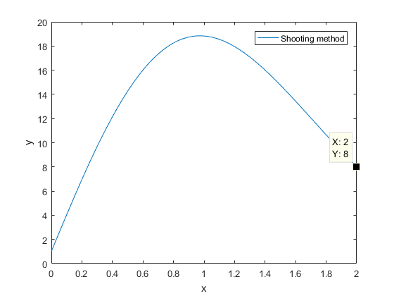

Shooting method in Python

We will solve the problem defined by Eqs. (8). The algorithm is basically the same as for Matlab and the structure of the program is also similar. First, let’s import necessary libraries. We will use odeint from scipy library for integrating differential equations, fsolve from the same library for finding solution of algebraic equation describing the boundary condition and matplotlib for plotting a diagram.

Python

import numpy as np
import matplotlib.pyplot as plt
from scipy.integrate import odeint
from scipy.optimize import fsolve

The function with right-hand sides of the system of ODEs is following:

Python

def rhs(y,x):
    dy = np.zeros(2)
    dy[0] = y[1]
    dy[1] = -x * y[1] - 2 * y[0]
    return dy

Please note, that the indexing in arrays starts from 0 in opposite to Matlab, where the first element has an index 1. Obviously, there are more differences, related to the characteristics of the programing languages. For example, in Python square brackets are, while round brackets are used in Matlab, and so on. Next, let’s write the function with algebraic equation for boundary condition:

Python

def bc(x):
    YY = odeint(rhs,[1, x[0]], np.linspace(0, 2, 100))
    y1_right=YY[-1,0]
    y2_right=YY[-1,1]
    F = y1_right-8
    return F

The function finding the unknown initial condition:

Python

def shoot_find():
    x = fsolve(bc, 1e-6)
    Y = odeint(rhs,[1, x[0]],np.linspace(0, 2, 100))
    return Y

The function running the above code and plotting the diagram:

Python

def shoot_method_problem_1():
    X = np.linspace(0, 2, 100)
    Y = shoot_find()
    plt.plot(X, Y[:, 0], label='Shooting method')
    plt.legend()
    plt.xlabel('x')
    plt.ylabel('y')
    plt.show()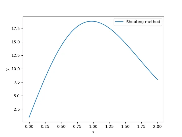

Diffusion-reaction process in a catalyst pellet

Definition of the problem

One of important problems in chemical engineering is modelling of catalyst pellet. The process for a flat geometry is described by second-order differential equation:

(9) $\frac{d^2C}{dx^2}-k C^n=0$

The boundary conditions related to this equation are following:

(10a) $\frac{dC(0)}{dx}=0$

(10b) $C(L)=C_L$

The first boundary condition denotes that at the catalyst bottom (x = 0) there is no mass transfer. Whereas at the catalyst surface (x = L) the concentration is known and equals C_L. We can see that it is a two-point boundary value problem, as the places where conditions are specified are different.

Transformation to the system

The second-order differential equation needs to be transformed to a system of first-order differential equations. First, let’s substitute C by y₁. Then we introduce variable y₂:

(11) $y_2=\frac{dy_1}{dx}$

After differentiation:

(12) $\frac{dy_2}{dx}=\frac{d^2y_1}{dx^2}$

After introducing y₂ and dy₂/dx into Eq. (9) we get:

(13) $\frac{dy_2}{dx}-k y_1^n=0$

Finally, the system of two first-order ODEs is:

(14a) $\frac{dy_1}{dx}=y_2$

(14b) $\frac{dy_2}{dx}=k y_1^n$

with boundary conditions:

(15a) $y_2(0)=0$

(15b) $y_1(L)=C_L$

Solution by the shooting method in Matlab

The procedure of finding the solution using shooting is the same as in problem defined by Eqs. (4). Now, we have two ODEs (14). At x = 0 one boundary is specified for y₂, while the other one, that is for y₁, is to be found. The condition for y₁(L) is known, so it will be used to verify, if the y₁(0) is chosen correctly.

The first function defines the right-hand sides of the system of ODEs.

MATLAB


function dy = rhs(x,y)
    dy = zeros(2,1);
    n = 2;
    k = 0.07;
    dy(1) = y(2);
    dy(2) = k * (y(1))^n;
end

The next function defines the boundary condition, as below:

MATLAB

function F = bc(x)
    CL = 0.05;
    options = optimoptions('fsolve','TolX',1e-8,'TolFun',1e-10');
    [X,YY] = ode45(@rhs,[0 20],[x 0],options);
    s=size(YY);
    y1_right=YY(s(1),1);
    F = [y1_right-CL];
end

MATLAB

function [X,Y]=shoot_find()
    options = optimoptions('fsolve','TolX',1e-8,'TolFun',1e-6');
    x = fsolve(@bc,0.001,options);
    [X,Y]=ode45(@rhs,[0:0.01:20],[x 0],options);
end

The shoot_find function executes the shoot_method and plots the result, as below.

MATLAB

function shoot_method_catalyst()
    [X,Y]=shoot_find();
    plot(X,Y(:,1))
    legend('Concentration distribution')
    xlabel('x')
    ylabel('C')
end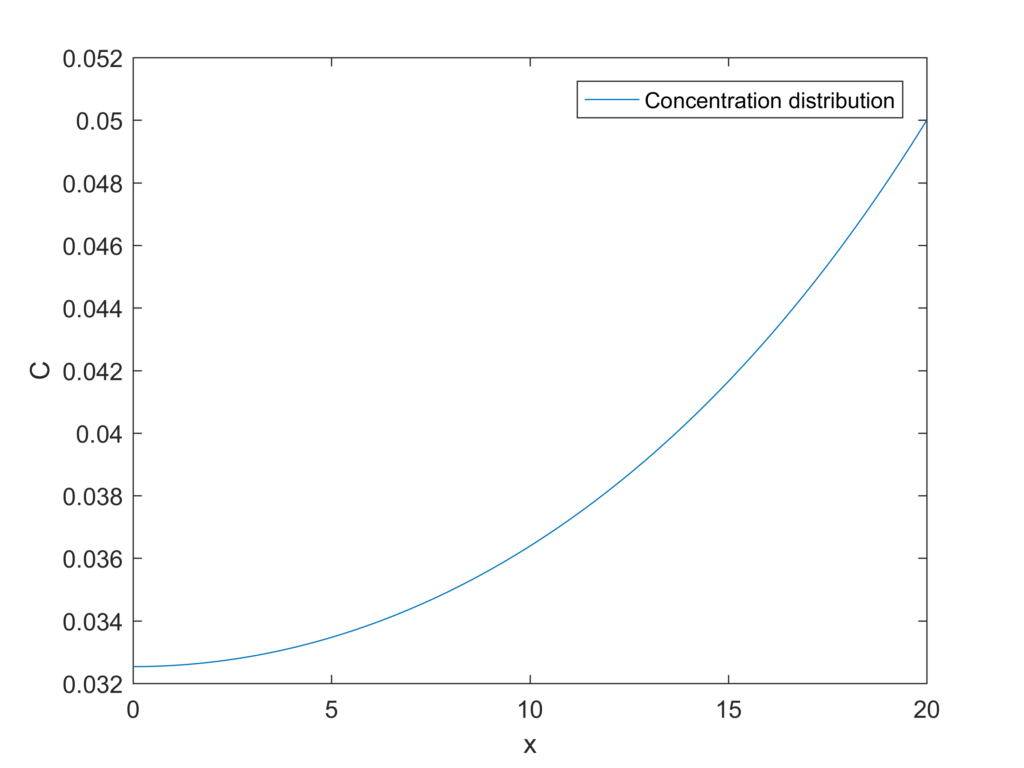

Fig. 4. Substrate concentration profile obtained using shooting method in Matlab

Solution by the shooting method in Python

The function with right-hand sides of the system of ODEs (14) is following:

Python

def rhs(y,x):
    n = 2
    k = 0.07
    dy = np.zeros(2)
    dy[0] = y[1]
    dy[1] = k * (y[0])**n
    return dy

Python

def bc(x):
    CL = 0.05
    YY = odeint(rhs,[x[0], 0], np.linspace(0, 20, 100))
    y1_right=YY[-1,0]
    F = y1_right-CL
    return F

The function finding the unknown initial condition:

Python

def shoot_find():
    x = fsolve(bc, 0.001)
    Y = odeint(rhs,[x[0], 0],np.linspace(0, 20, 100))
    return Y

The function running the above code and plotting the diagram:

Python

def shoot_method_catalyst():
    X = np.linspace(0, 2, 100)
    Y = shoot_find()
    plt.plot(X, Y[:, 0], label='Concentration distribution')
    plt.legend()
    plt.xlabel('x')
    plt.ylabel('C')
    plt.show()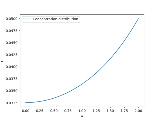

Fig. 5. Substrate concentration profile obtained using shooting method in Python

Summary

Shooting method is a simple and effective method for solving boundary value problems. In the article, an exemplary second-order differential equation was solved using Matlab and Python. The model of a catalyst pellet described by diffusion-equation was also solved.

References

[1] http://www.scholarpedia.org/article/Boundary_value_problem

[2] Press, William H. Numerical recipes 3rd edition: The art of scientific computing. Cambridge university press, 2007.

Shooting method – boundary value problem in Matlab and Python

What is a shooting method?

Shooting method in Matlab

Shooting method in Python

Diffusion-reaction process in a catalyst pellet

Definition of the problem

Transformation to the system

Solution by the shooting method in Matlab

Solution by the shooting method in Python

Summary

References