This is a part of Lecture notes in process control
Introduction
Process dynamics concerns the dynamic behavior of various industrial processes and devices. The production rate and the quality of the product depend on the operating conditions, such as temperature, pressure, energy input, etc. (Rohani, 2017). Control is to maintain desired conditions in a system by adjusting selected input variables of the system. Process control can range from simple manual actions to computer logic controllers, remote from the required action point, with supplemental instrumentation feedback systems.
The objectives of process control are, among others (Berk, 2018):
- To enhance the reliability of the process.
- To improve process safety.
- To increase production.
- To reduce the proportion of production units that do not meet the specifications.
- To improve process economics by reducing production costs.
Depending on whether a person (an operator) is physically involved in the control system, control systems are divided into manual control systems and automatic control systems. Early machines were all manually operated. Many machines are still manually controlled, but almost all machines incorporate elements of automation.
Examples of manual control
Examples of manual control systems are presented in Fig. 1. The drawing to the left presents a situation in which the operator regulates the level of liquid by adjusting the output valve. The operator compares the actual level with the desired level and opens or closes the valve. The drawing to the right illustrates the situation in a man regulates the temperature of water. To start the heating process, the valve in the hot water line is opened. The operator can then determine the effectiveness of the control process by standing and measuring (manually) the temperature. If the water is too hot, the valve should be closed a little or even turned off. If the water is not hot enough, then the valve is left open or opened wider.
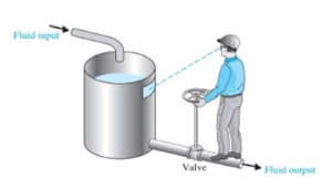

Fig. 1 Examples of manual control systems
Based on the second example, we can easily set up an automatic control system, as shown in Fig. 2. Firstly, a temperature measurement device is used to measure the water temperature, which replaces the operator’s hand. This addition to the system improves accuracy. Instead of a manual valve, a special kind of valve, called a control valve, is used that is driven by compressed air or electricity. A device called a controller, in this case a temperature controller, is used to replace the brain of the operator. This has the function of comparing the actual and desired temperature and giving required orders to the control valve.

Process Control Terminology
- Controlled variables – these are the variables that quantify the performance or quality of the final product, which are also called output variables.
- Manipulated variables – these input variables are adjusted dynamically to keep the controlled variables at their set points.
- Disturbance variables – these are also called “load” variables and represent input variables that can cause the controlled variables to deviate from their respective set points.
Examples of process dynamics
Fig. 3 shows a tank into which a liquid is pumped at a variable rate, FVf (m3/s). The subscript ‘f’ will be used to denote the feed stream. This inflow rate can vary with time because of changes in the process. The height of the liquid in the vertical cylindrical tank is h (m). The flow rate out of the tank is FV (m3/s). FVf, h, and FV will all vary with time and are therefore functions of time t. Liquid leaves the base of the tank via a long horizontal pipe.
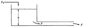
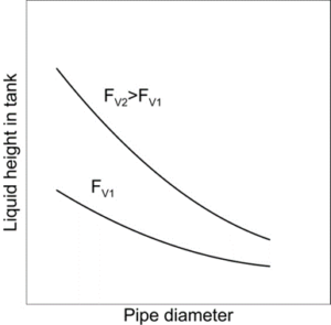
Let us first look at the steady-state conditions. By steady-state, we mean, in most systems, the conditions when nothing is changing with time. Mathematically, this corresponds to having all time derivatives equal to zero, or to allowing time to become very large, i.e., go to infinity. At a steady state the flow rate out of the tank must equal the flow rate into the tank: FVf* = FV*(an asterisk will be used to denote steady state). For a given FVf*, the height of liquid in the tank at steady-state would also achieve constant value h*. The liquid height provides hydraulic pressure at the inlet of the pipe to overcome the frictional pressure losses of the liquid flowing through the pipe. The steady-state design of the tank involves the selection of the height and diameter of the tank and the diameter of the exit pipe. For a given pipe diameter, the tank height must be large enough to prevent the tank from overflowing at the maximum expected flow rate. A larger pipe diameter requires a lower liquid height, as illustrated in Fig. 4.
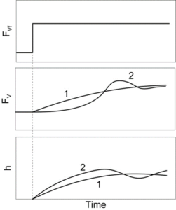
But what paths will h(t) and FV(t) take to get to their new steady-states? Fig. 5 illustrates the problem. The question is which curves (1 or 2) represent the actual paths (also called time trajectories) that FV(t) and h(t) will follow. Curves 1 show gradual increases in h(t) and FV(t) to their new steady-state values. However, the paths could follow curves 2, where the liquid height rises above its final steady-state value. This is called “overshoot”. It is necessary to derive a mathematical model of the system to determine its dynamic response quantitatively through simulation. This will be the subject of further lectures.
A dynamic simulation of a flow-gravity tank can be found here:
https://demonstrations.wolfram.com/DynamicSimulationOfAGravityFlowTank
Check also:
REFERENCES
Berk, Z., 2018. Food process engineering and technology. Academic Press.
Luyben, W.L., 1989. Process modeling, simulation and control for chemical engineers. McGraw-Hill Higher Education, New York-Toronto.
Rohani, S., 2017. Coulson and Richardson’s Chemical Engineering: Volume 3B: Process Control. Butterworth-Heinemann.
Rowe, W.B., 2013. Principles of modern grinding technology. William Andrew.