This is a part of the lecture notes in process control.
Equilibrium
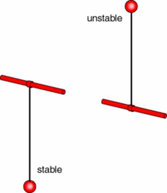
Equilibrium of a dynamical system is a state that does not change with time. For example, each motionless pendulum position in Fig. 1 presents an equilibrium. One of them is stable, the other one is unstable. An equilibrium is considered stable if the system returns to the original point after small disturbances. If the system moves away from the equilibrium after small disturbances, then the equilibrium is unstable.
Consider the following ordinary differential equation:
(1) ![\[\frac{dx}{dt}=f(x)\]](https://softinery.com/wp-content/ql-cache/quicklatex.com-ec73ce08fc1dd9b0fac6717e497a6448_l3.png "Rendered by QuickLaTeX.com")
where:
![\[x=\left[ \begin{matrix} {{x}_{1}} \\ {{x}_{2}} \\ ... \\ {{x}_{n}} \\ \end{matrix} \right]\,\ ,\quad \quad f=\left[ \begin{matrix} {{f}_{1}} \\ {{f}_{2}} \\ ... \\ {{f}_{n}} \\ \end{matrix} \right]\]](https://softinery.com/wp-content/ql-cache/quicklatex.com-afdb9f9011d4a22e55d41189664d5115_l3.png "Rendered by QuickLaTeX.com")
The Equation (1) has an equilibrium solution  if
if  . An equilibrium is also called a steady state. There are methods that can be used to predict the stability of a system based on calculations.

The stability of an equilibrium is determined by the sign of real part of eigenvalues of the Jacobian matrix. The Jacobian matrix of a system of ordinary differential equations (ODEs) is the matrix of the partial derivatives of the right-hand side with respect to state variables:
(2) ![\[J=\left[ \begin{matrix} \frac{\partial {{f}_{1}}}{\partial {{x}_{1}}} & \frac{\partial {{f}_{1}}}{\partial {{x}_{2}}} & \ldots & \frac{\partial {{f}_{1}}}{\partial {{x}_{n}}} \\ \frac{\partial {{f}_{2}}}{\partial {{x}_{1}}} & \frac{\partial {{f}_{2}}}{\partial {{x}_{2}}} & \ldots & \frac{\partial {{f}_{2}}}{\partial {{x}_{n}}} \\ \ldots & \vdots & \ddots & \vdots \\ \frac{\partial {{f}_{n}}}{\partial {{x}_{1}}} & \frac{\partial {{f}_{n}}}{\partial {{x}_{2}}} & \ldots & \frac{\partial {{f}_{n}}}{\partial {{x}_{n}}} \\ \end{matrix} \right]\]](https://softinery.com/wp-content/ql-cache/quicklatex.com-a81f760317ba8a3b6217dc6b98f537d3_l3.png "Rendered by QuickLaTeX.com")
where all derivatives are evaluated at the equilibrium point  .
.
To obtain eigenvalues of Jacobain matrix it is necessary to solve a characteristic equation:
(3) ![\[\det (J-\mu I)=0\]](https://softinery.com/wp-content/ql-cache/quicklatex.com-458df8f868b4708bb623c60e44eb990c_l3.png "Rendered by QuickLaTeX.com")
where I is a unit matrix and μ is eigenvalue.
We will consider two-dimensional system, i.e. a system described by two state variables: x1 and x2. According to Eq. (1) we have:
(4a) ![\[\frac{d{{x}_{1}}}{dt}={{f}_{1}}({{x}_{1}},{{x}_{2}}) \]](https://softinery.com/wp-content/ql-cache/quicklatex.com-674bd201710502a65bc51238d0315096_l3.png "Rendered by QuickLaTeX.com")
(4b) ![\[\frac{d{{x}_{2}}}{dt}={{f}_{2}}({{x}_{1}},{{x}_{2}}) \]](https://softinery.com/wp-content/ql-cache/quicklatex.com-80356cb38c3ed6c0dac42261e31223ad_l3.png "Rendered by QuickLaTeX.com")
The Jacobian matrix has the form:
(5) ![\[J=\left[ \begin{matrix} \frac{\partial {{f}_{1}}}{\partial {{x}_{1}}} & \frac{\partial {{f}_{1}}}{\partial {{x}_{2}}} \\ \frac{\partial {{f}_{2}}}{\partial {{x}_{1}}} & \frac{\partial {{f}_{2}}}{\partial {{x}_{2}}} \\ \end{matrix} \right] \]](https://softinery.com/wp-content/ql-cache/quicklatex.com-8e1eb3d4d59f63de779284ce0b5ada6d_l3.png "Rendered by QuickLaTeX.com")
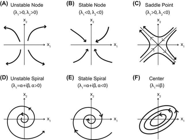
It has two eigenvalues, which are either both real or complex-conjugate. An equilibrium can be a
- Node when both eigenvalues are real and of the same sign. The node is stable when the eigenvalues are negative and unstable when they are positive.
- Saddle when eigenvalues are real and of opposite signs. The saddle is always unstable.
- Focus (called spiral point) when eigenvalues are complex-conjugate. The focus is stable when the eigenvalues have negative real part and unstable when they have positive real part.
- Limit cycle (called center) if eigenvalues are imaginary and have zero real parts.
As we already know from previous lecture, it is convenient to illustrate result on a phase plane. One reason for that it each type of equilibrium will shape differently, what simplifies analysis. Let’s remind that for a simple pendulum model we obtained a closed curve on a phase plane, i.e. a limit cycle. This type of equilibrium and other ones are illustrated in Fig. 2. Arrows on curves indicate the direction of time. As we can see if the equilibrium is stable, then with time the system tends to a certain point. This point represents equilibrium.
Summary
Stability analysis is an important subject in process engineering. It is used to determine the behavious of a dynamic system in an equilibrium point. You could read in the article how to perform stability analysis based on the system of differential equations describing the system and Jacobian matrix.
REFERENCES
Chou, C.-S., & Friedman, A. (2016). System of Two Linear Differential Equations BT – Introduction to Mathematical Biology: Modeling, Analysis, and Simulations (C. S. Chou & A. Friedman (Eds.); pp. 29–42). Springer International Publishing. https://doi.org/10.1007/978-3-319-29638-8_3
Izhikevich, E. M. (2007). Equilibrium. Scholarpedia, 2(10).