Plug-flow reactor model
Plug-flow reactor (PFR, sometimes called piston-flow reactor or tubular reactor) is an idealized reactor in which all particles in a given cross-section have identical velocity and direction of motion. In PFR there is no mixing or back flow, so the fluid flows like a plug, from inlet to outlet (Figure below).
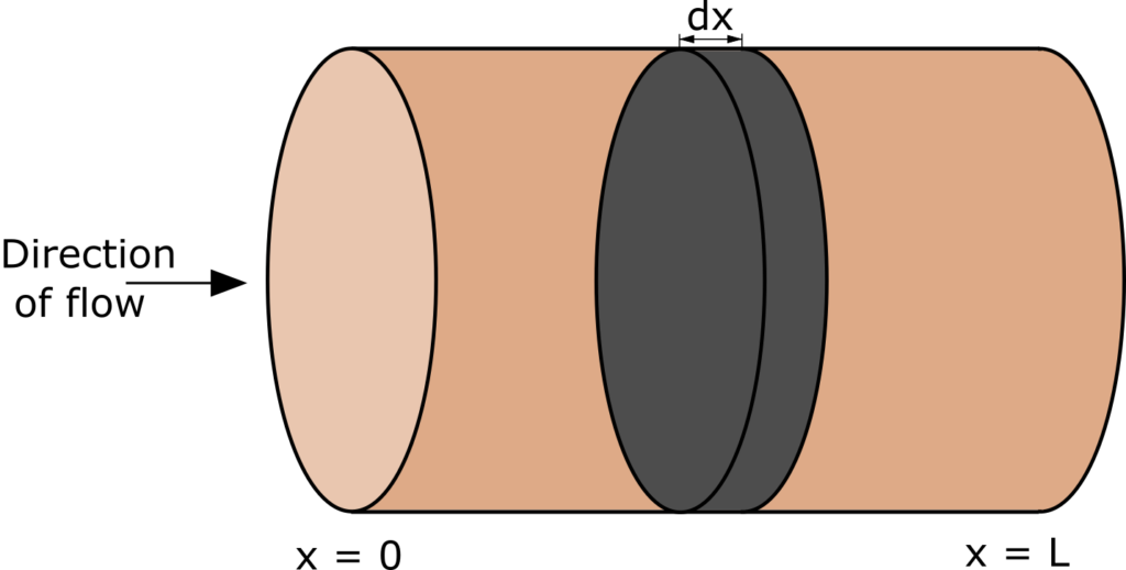
Plug flow reactor model is formulated based on mass balance and heat balance in a differential volume of a fluid (Fig. 1). If we assume that the process is isothermal (heat of reaction is negligible), then only mass balance is considered. We will assume steady state conditions, which mean that concentrations of reactant do not change over time. It is a typical way of operation of plug flow reactors.
The mathematical model of PFR can be written as follows (Levenspiel, 1998):
![\[u\frac{dC_{i}}{dx}=v_{i}}r\]](https://softinery.com/wp-content/ql-cache/quicklatex.com-fee4efe7f9b627554f17ba58244338e3_l3.png "Rendered by QuickLaTeX.com")
![\[C_{i}(0)=C_{if}\]](https://softinery.com/wp-content/ql-cache/quicklatex.com-c99dd4432bee0129ce2a2eb2ea5f9660_l3.png "Rendered by QuickLaTeX.com")
![\[0\le x\le L\]](https://softinery.com/wp-content/ql-cache/quicklatex.com-c24e41832914845acefe4ae57db0051d_l3.png "Rendered by QuickLaTeX.com")
In the above equation Ci is reactant i concentration, u denotes fluid velocity, νi is the stoichiometric coefficient, r is the reaction rate and x is the position in the reactor. Caf is reactant A concentration at the reactor inlet (in the feed stream) and L is the reactor length.
The fluid velocity u is calculated based on the volumetric flow rate Fv (m3/s) and the cross-section area of the reactor S (m2):
![\[u=F_v/S\]](https://softinery.com/wp-content/ql-cache/quicklatex.com-ab28801b7c23391100ca879fc8f34e67_l3.png "Rendered by QuickLaTeX.com")
In an ideal plug flow reactor, all the fluid particles have been inside the reactor for exactly the same amount of time (Fogler, 2010). We call this value a mean residence and calculate as
![\[\tau=L/u\]](https://softinery.com/wp-content/ql-cache/quicklatex.com-9acd2259568080666afdf036f463d0a4_l3.png "Rendered by QuickLaTeX.com")
The residence time data is commonly used in chemical reactors engineering to make predictions of conversion and exit concentrations.
First-order irreversible reaction
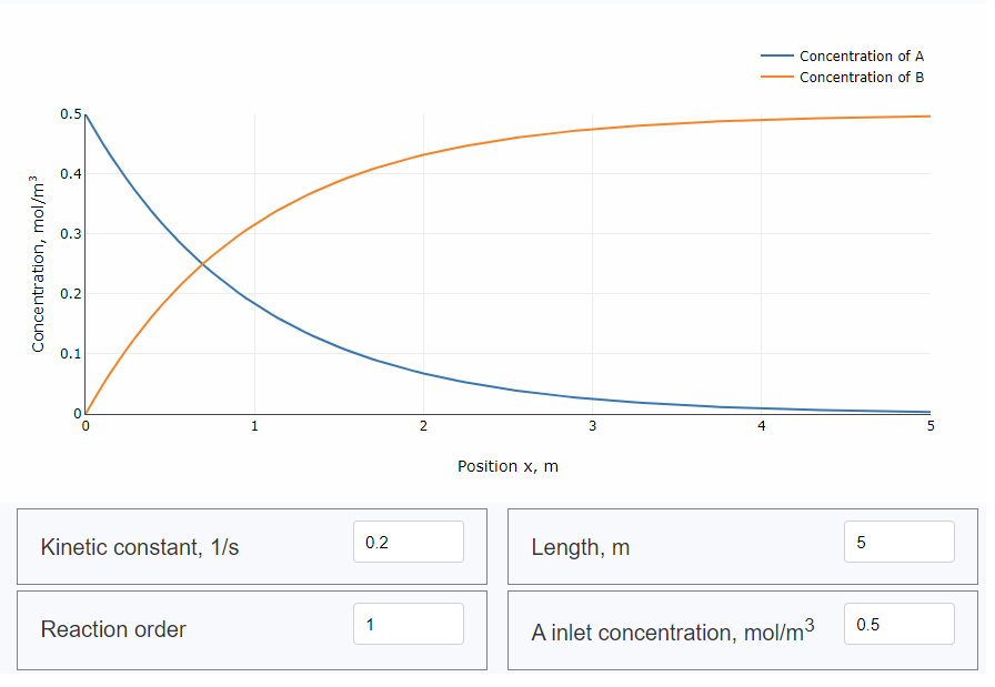
Let’s consider simple decomposition reaction:
![\[A\to 2B\]](https://softinery.com/wp-content/ql-cache/quicklatex.com-8a2fa6f3a0c1081c348ead412d952d66_l3.png "Rendered by QuickLaTeX.com")
When the reaction is irreversible and first-order, then we have:
![\[u\frac{dC_{a}}{dx}=-kC_{a}\]](https://softinery.com/wp-content/ql-cache/quicklatex.com-dedc3a9a166d0b754130eb25a2bb2312_l3.png "Rendered by QuickLaTeX.com")
where k is a kinetic constant. In general, kinetic constant depends on temperature. Commonly an Arrhenius equation is used to describe this relationship. Here, we assume isothermal conditions, so will not use this dependency.
For first-order irreversible reaction, the model can be solved analytically. The solution is following:
![\[C_{a}=C_{af}exp(-x*k/u)\]](https://softinery.com/wp-content/ql-cache/quicklatex.com-7f1eedea226ab1ab9bb367b7f615b953_l3.png "Rendered by QuickLaTeX.com")
Second-order irreversible reaction
As an example of a second-order irreversible reaction, let’s use the following one:
![\[2A\to B\]](https://softinery.com/wp-content/ql-cache/quicklatex.com-ffc9bdc8cf43353b3d89a4543168e17a_l3.png "Rendered by QuickLaTeX.com")
When the reaction is irreversible and second-order, then we have:
![\[u\frac{dC_{a}}{dx}=-2k*(C_{a})^2\]](https://softinery.com/wp-content/ql-cache/quicklatex.com-fcd29d10ede86d08827f2c00df26ba7b_l3.png "Rendered by QuickLaTeX.com")

Simulation of plug flow reactor
First-order reaction
First, let’s import necessary libraries: numpy for matrix operations, scipy for solving differential equations and matplotlib for making a chart.
import numpy as np
from scipy.integrate import odeint
import matplotlib.pyplot as plt
Next, we will define reaction function. In this example we use first-order irreversible reaction.
def reaction(ca, k):
  r = k * ca
  return r
The function plug_flow describes the differential equation.
def plug_flow(ca, x, k, ni, u):
  r = reaction(ca, k)
  dcadx = ni * r / u
  return dcadx
Snippet below presents the definition of model parameters.
# kinetic constant
k = 0.1
# reactor length
L = 10
x = np.linspace(0, L, 101)
ca0 = 0.6
ni = -1
u = 0.5
Next, we will use odeint function from scipy library to solve the differential equation.
sol = odeint(plug_flow, ca0, x, args=(k, ni, u))Finally, we will plot the results together with the analytical solution for the comparison.
plt.plot(x, sol)
plt.plot(x[::4], [ca0 * np.exp(-x*k/u) for x in x[::4]],'o')
plt.xlabel('x')
plt.ylabel('$C_{a}$')
plt.legend(['numerical', 'analytical'])
plt.plot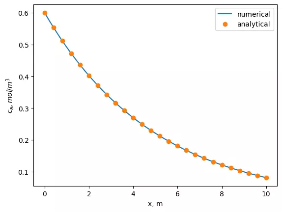
Second-order reaction
Obtaining the solution is very similar. We need to change the reaction function and coefficient ν. The final code looks as follows:
import numpy as np
from scipy.integrate import odeint
import matplotlib.pyplot as plt
def reaction(ca, k, n):
  r = k * ca ** n
  return r

def plug_flow(ca, x, k, ni, u, n):
  r = reaction(ca, k, n)
  dcadx = ni * r / u
  return dcadx

# kinetic constant
k = 0.1
# reactor length
L = 10
x = np.linspace(0, L, 101)
# inlet A concentration
ca0 = 0.6
# reaction order
n = 2
# stoichiometric coefficient
ni = -2
# fluid velocity
u = 0.5

sol = odeint(plug_flow, ca0, x, args=(k, ni, u, n))

plt.plot(x, sol)
plt.xlabel('x, m')
plt.ylabel('$c_a, mol/m^3$')
plt.legend(['numerical'])
plt.plot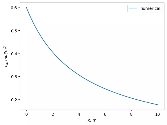
References
Try online plug-flow reactor simulator
Read related content
How to solve system of DAEs in Python