Mathematical modelling

This is a part of the lecture notes in process control.

Introduction

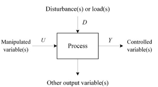
A mathematical relationship between the input and output variables in which time is independent is referred to as the dynamic model of the process. A dynamic model can be developed based on the first principles, i.e., mass, energy, momentum, etc., balances or based on an empirical approach using the input–output data of the process.

Fig. 1 The block diagram of a typical process with the designated input and output variables (Rohani, 2017)

Example of a mathematical model: a pendulum

Description of the system

Let us consider an idealized pendulum (called a simple pendulum). This is a weight on the end of a massless cord suspended from a pivot point P. In this model, there is no frictional energy loss. The pendulum will swing back and forth with periodic motion.

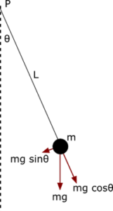
By applying Newton’s second law, the dynamical equation of motion for the pendulum may be obtained:

(1) $\frac{{{d}^{2}}\theta }{d{{t}^{2}}}+\frac{g}{L}\theta =0$

with initial conditions:

(2a) $\theta (0)={{\theta }_{0}}$

(2a) $\frac{d\theta (0)}{dt}=0$

Where θ is the angle (angular displacement), L is the length of the cord, and g is acceleration due to gravity. At the initial moment, the angular displacement is equal to θ₀, and the velocity is equal to zero. The above mathematical model can be used to determine the pendulum behavior, in this case the angular displacement with time. To this end, the differential Eq. (1) should be solved.

The solution of a pendulum model

There are several methods that can be used, for example, the method based on the Laplace transform (this one will be described in one of the next lectures). Here, we will utilize Matlab computing software. Detailed information on the procedure used can be found in the documentation:

https://in.mathworks.com/help/symbolic/dsolve.html

The Matlab script solve_pendulum.m, which solves the differential equation is attached to this lecture.

MATLAB

syms L g t theta(t) theta0
dtheta=diff(theta,t);
ts = dsolve(diff(theta,t,2)+theta*g/L==0,theta(0)==theta0,dtheta(0)==0);
ts = simplify(ts)

The solution obtained is the following:

(3) $\theta (t)={{\theta }_{0}}\cos \left( \sqrt{\frac{g}{L}}\cdot t \right)$

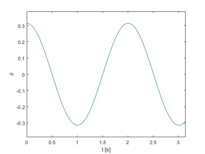
Now, using the solution, we can see how the angular displacement will change over time. To get real numbers, we have to set the values of the model parameters (i.e. the values that are constant: g and L in this case) and the initial condition θ₀. The length will equal 1 m, while θ₀ = π/10. Different values can be used, depending on the characteristics of the pendulum. The obtained relationship θ(t) is illustrated in Fig. 3. As could be expected, the displacement is changing periodically. We should notice that according to this mathematical model, the pendulum will swing infinitely long, as friction was neglected. In order to obtain more realistic results, a more detailed model has to be used.

At this point, it is necessary to introduce the definition of a state variable. A state variable is one of the variables that are used to describe the mathematical state of a dynamical system. In this example, θ is a state variable. It is possible that a dynamical system is described by more than one state variable.

Fig. 3 Illustration of dynamical changes in the angular displacement of a simple pendulum

The Matlab file Pendulum.m, which plots this diagram is also attached to this lecture.

MATLAB

syms t
g=sym(9.81);
l=sym(1);
theta0=sym(pi/10);
theta = theta0*cos(sqrt(g/l)*t);
gama=-theta0*sin(sqrt(g/l)*t)*sqrt(g/l);
figure(1) 
ezplot(theta,[0,pi])
xlabel('t [s]')
ylabel('\theta')
title('')
figure(2)
ezplot(gama,theta)
xlabel('\gamma')
ylabel('\theta')
title('')
figure(3)
subplot(2,1,1)
ezplot(theta,[0,pi])
xlabel('t [s]')
ylabel('\theta')
title('')
subplot(2,1,2)
ezplot(gama,[0,pi])
xlabel('t [s]')
ylabel('\gamma')
title('')

If you cannot use Matlab software, it is possible to go to the Wolfram Alpha website to see an online solver of this problem:

https://www.wolframalpha.com/input/?i=pendulum&lk=3

Transformation of a second-order ODE to a system of first-order ODEs

The presented model can also be used to get additional information about the velocity of the pendulum. However, some transformations are required. Eq. (1) is a second-order differential equation. It can be transformed into a system of two differential equations of first order. To this end, we need to introduce the additional variable γ:

(4) $\gamma =\frac{d\theta }{dt}$

As you can see, γ is the angular velocity, i.e. the change of angular displacement over time. If we derivate the above equation., then we get:

(5) $\frac{d\gamma }{dt}=\frac{{{d}^{2}}\theta }{{{d}^{2}}t}$

Now, we will introduce a new variable and its derivative to Eq. (1). The system obtained as follows:

(6) $\frac{d\gamma }{dt}+\frac{g}{L}\theta =0$

We obtained a system of two differential equations. Let’s rewrite it below:

(7a) $\frac{d\theta }{dt}=\gamma$

(7b) $\frac{d\gamma }{dt}+\frac{g}{L}\theta =0$

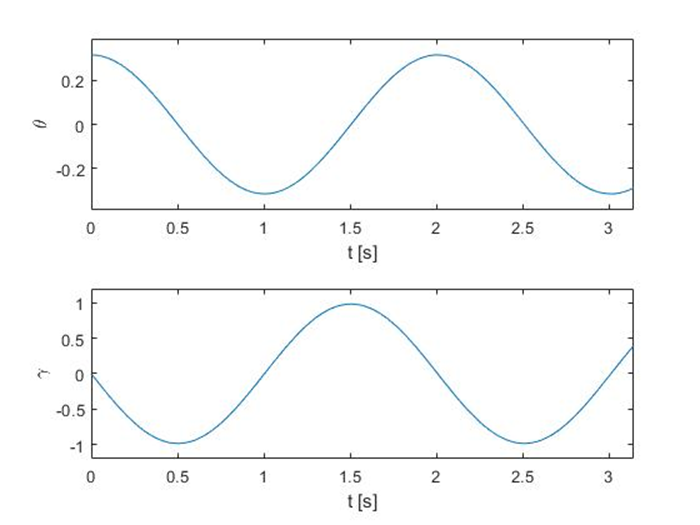
We can notice that the system is now described by two state variables: γ and θ. As before, the model should be solved. At this point, we will omit the method of solving the system of differential equations. The solution is following:

(8a) $\theta (t)={{\theta }_{0}}\cos \left( \sqrt{\frac{g}{L}}\cdot t \right)$

(8b) $\gamma (t)=-{{\theta }_{0}}\sin \left( \sqrt{\frac{g}{L}}\cdot t \right)\sqrt{\frac{g}{L}}$

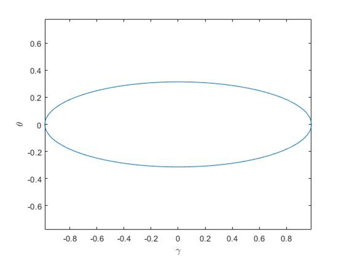
The solution is illustrated in Fig. 4. It is sometimes more convenient to show the results in a different manner. Figure 5 presents a phase trajectory. In simple words, it is a curve representing relationship between one state variable and another. The diagram at which coordinates corresponds to state variables is a phase plane. The trajectory shows how the state of a dynamical system changes with time. A periodic solution, such us obtained in this example, gives a closed loop called a limit cycle.

REFERENCES

Rohani, S. (2017). Coulson and Richardson’s Chemical Engineering: Volume 3B: Process Control. Butterworth-Heinemann.