What is curve fitting?
Curve fitting is a method of finding a mathematical function that best fits data points. This method is often used in many fields of engineering, life-science or economics in situations where we want to find a relationship between two variables, preferably in the form y = f(x). Typically, the data we are dealing with is subject to some error, so the function does not have to go through all the points exactly. Instead, we search for an approximate function that describes the data series as a whole with the smallest error. One way to minimize the total error is to use the method of least squares. Below I will discuss the most common types of functions used, and then how to implement curve fitting in Python.
Linear regression
It is a type of statistical method used to find a linear relationship between two variables – independent and dependent one. This method is also called “simple linear regression”. There is also multiple linear regression – when the linear relationship is to be found between more than one independent variables and one dependent variable.
Polynomial fit
The relationship between the independent variable x and the dependent variable y is in the form of an nth degree polynomial of x.
We can categorize polynomial fit with respect to the degree:
- Linear – if degree is 1. The equation of fit curve is:

2. Quadratic – if degree is 2. The equation of fit curve is:

3. Cubic – if degree is 3. The equation of fit curve is:

and so on. The order of fitting polynomial can be generally n.
Exponential fit
In exponential fit the following equation is used:

An exponential function is used to describe processes with rapid growth of decay of some quantity. Examples include growth of bacteria, radioactive decay, chemical reaction kinetics.
Power fit
The following function is used for the power fitting:

Four parameters logistic regression
Four parameters logistic regression (4PL) is often used in modelling of many biological systems. As the result of fitting, S shaped curve is obtained. The formula used for fitting is following:

where:
a – the minimum value that can be obtained (y at x = 0)
b – Hill’s slope of the curve
c – the point of inflection (i.e. the point on the curve halfway between a and d)
d – the maximum value that can be obtained (y at x tending to infinity)
Implementation of curve fitting in python
We will start with importing libraries.
import numpy as np
from scipy import stats, polyfit
import sympy as sp
from scipy.optimize import curve_fit
from sklearn.metrics import r2_score
import matplotlib.pyplot as plt
Linear function
First, we will consider linear regression using linregress from scipy library. Let’s define a user-defined function (linreg) which calculates additional variables, useful for plotting and evaluation. It will return a dictionary with r squared, sum of squared error, parameters of the regression line and arrays for drawing a diagram.
def linreg(x,y):
    res = stats.linregress(x,y)

    xmin = min(x)
    xmax = max(x)

    # Data for plotting fitted line
    xreg = np.linspace(xmin, xmax)
    yreg = res.intercept + res.slope * xreg

    y_predicted = res.intercept + res.slope * x
    # Calculate SSE
    sse = calculate_sse(y, y_predicted)

    # Calculate r2

    r2 = res.rvalue ** 2
    # Calculate adjusted R-squared
    n = len(y)
    p = 2
    adjusted_R_squared = 1 - (1 - r2) * (n - 1) / (n - p - 1)

    return {'x': xreg, 'y': yreg, 'r2': r2, 'intercept': res.intercept, 'slope': res.slope, 'sse': sse,
            'adj_r2': adjusted_R_squared}
The code below is an example of using the above function.
x = np.array([5,7,8,7,2,17,2,9,4,11,12,9,6])
y = np.array([99,86,87,88,111,86,103,87,94,78,77,85,86])

linreg_data = linreg(x,y)
plt.scatter(x, y)
plt.plot(linreg_data['x'], linreg_data['y'])
plt.xlabel('x')
plt.ylabel('y')
plt.legend(['Data', 'Linear regression'])
plt.show()

print("R squared:", linreg_data['r2'])
Polynomial function
Next, let’s create a function for polynomial fit. Similarly as for linear regression, the function returns additional useful variables in the form of a dictionary. Polyfit is the core method below. It calculates the coefficients of the polynomial. They are afterwards used to create a polynomial function using poly1d from numpy library.
def poly(x,y,degree):

    # Perform polynomial fit using scipy's polyfit
    coefficients = polyfit(x, y, degree)

    # Create a polynomial function using the coefficients
    polynomial_function = np.poly1d(coefficients)

    # Generate x values for plotting the fitted curve
    x_fit = np.linspace(min(x), max(x), 40)

    # Calculate y values using the fitted curve
    y_fit = polynomial_function(x_fit)

    # Calculate R-squared (coefficient of determination)
    y_predicted = polynomial_function(x)
    r2 = r2_score(y, y_predicted)

    # Calculate SSE
    sse = calculate_sse(y, y_predicted)

    xmin = min(x)
    xmax = max(x)

    # Calculate adjusted R-squared
    n = len(y)
    p = len(coefficients)
    adjusted_R_squared = 1 - (1 - r2) * (n - 1) / (n - p - 1)

    return {'x': x_fit, 'y': y_fit, 'r2': r2, 'coefficients': coefficients, 'sse': sse,
            'adj_r2': adjusted_R_squared}
Let’s use the function created to make a fit to previously defined x and y arrays.
poly_data = poly(x,y, 2)
plt.scatter(x, y)
plt.plot(poly_data['x'], poly_data['y'])
plt.xlabel('x')
plt.ylabel('y')
plt.legend(['Data', 'Polynomial regression'])
plt.show()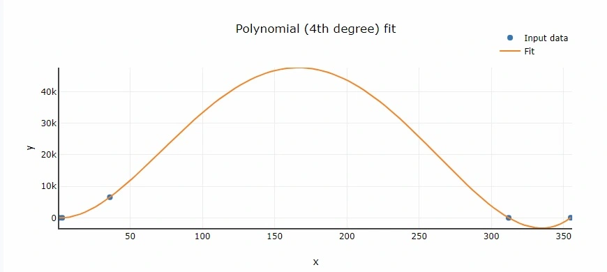
Online Curve Fitting Tool
Exponential function
The function presented below is slightly different than the ones created previously. Here, we use curve_fit method from scipy library. We can use it for fit of any function defined by the programmer. Here we use exponential function.
def fit_expon(x,y):

    # Perform the curve fit

    popt, pcov = curve_fit(exponential_func, x, y, p0=[1.44, 0.35], maxfev=5000)

    # Extract the optimized parameters
    a_opt, b_opt = popt

    # Generate fitted values for plotting
    x_fit = np.linspace(min(x), max(x), 40)
    y_fit = exponential_func(x_fit, a_opt, b_opt)

    # Calculate the predicted values of y using the fitted parameters
    y_predicted = exponential_func(x, a_opt, b_opt)

    # Calculate R-squared (coefficient of determination)
    r2 = r2_score(y, y_predicted)

    # Calculate SSE
    sse = calculate_sse(y, y_predicted)

    # Calculate adjusted R-squared
    n = len(y)
    p = len(popt)
    adjusted_R_squared = 1 - (1 - r2) * (n - 1) / (n - p - 1)

    return {'x': x_fit, 'y': y_fit, 'r2': r2, 'coefficients': popt, 'sse': sse,
            'adj_r2': adjusted_R_squared}

def exponential_func(x, a, b):
    return a * np.exp(b * x)
Let’s take a look at the line with curve_fit:
popt, pcov = curve_fit(exponential_func, x, y, p0=[1.44, 0.35], maxfev=5000)
We see that it accepts several arguments: the fitted function (exponential_func), arrays with data (x and y), initial guess (p0) and maximum number of evaluations (maxfev). The initial guess represents values from which the calculations will be started. The curve_fit returns two variables: popt and pcov:
- popt : estimated values for parameters of best-fit curve,
- pcov: covariance matrix or errors.
For the exponential fit above we get:
popt = [3.5351332 0.47297806, 0.47297806]
and
pcov = [[ 9.83726219e-02 -2.83133970e-03] [-2.83133970e-03 8.22300127e-05]]
The code below shows how to perform the curve fitting for exponential function using example dataset and plot the fitted curve using matplotlib.
x = np.array([1, 2, 3, 6, 7, 10])
y = np.array([2, 7, 10, 60, 100, 400])
expon_data = fit_expon(x,y)
plt.scatter(x, y)
plt.plot(expon_data['x'], expon_data['y'])
plt.xlabel('x')
plt.ylabel('y')
plt.legend(['Data', 'Exponential fit'])
plt.show()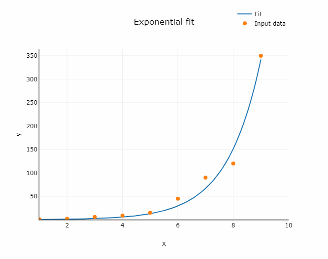
Power function
Analogically to the code in above section, we can use any other user-defined mathematical function. Example below shows power function.
def fit_power(x,y):

    # Perform the curve fit

    popt, pcov = curve_fit(power_func, x, y, p0=[1.44, 0.35], maxfev=5000)
    # popt, pcov = curve_fit(lambda t, a, b, c: a * np.exp(b * t) + c, x, y)

    # Extract the optimized parameters
    a_opt, b_opt = popt

    # Generate fitted values for plotting
    x_fit = np.linspace(min(x), max(x), 40)
    y_fit = power_func(x_fit, a_opt, b_opt)

    # Calculate the predicted values of y using the fitted parameters
    y_predicted = power_func(x, a_opt, b_opt)

    # Calculate R-squared (coefficient of determination)
    r2 = r2_score(y, y_predicted)

    # Calculate SSE
    sse = calculate_sse(y, y_predicted)

    # Calculate adjusted R-squared
    n = len(y)
    p = len(popt)
    adjusted_R_squared = 1 - (1 - r2) * (n - 1) / (n - p - 1)

    return {'x': x_fit, 'y': y_fit, 'r2': r2, 'coefficients': popt, 'sse': sse,
            'adj_r2': adjusted_R_squared}


def power_func(x, a, b):
    return a * x ** b
Sum of squared error
The sum of squared error (SSE) is the total squared difference between the observed y-values and the y-values predicted by the model. It provides an measure of how well the model fits the data points. Let’s see the code for calculating the sum of squared error.
def calculate_sse(y_actual, y_predicted):
    # Convert the input lists to NumPy arrays for vectorized operations
    y_actual = np.array(y_actual)
    y_predicted = np.array(y_predicted)

    # Calculate squared errors and sum them up
    squared_errors = (y_actual - y_predicted) ** 2
    sse = np.sum(squared_errors)

    return sse
Summary
Curve fitting is a significant method both in data analysis, machine learning and data science. It plays a crucial role in understanding relationships between variables, making predictions, and extracting insights from data. In this article read how to implement curve fit using scipy library. In particular, you learned how to:
- implement linear, polynomial, exponential and power fit,
- calculate R squared, adjusted R squared and sum of squared error.
Related content
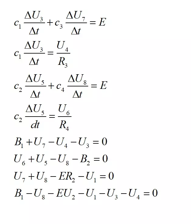
How to solve system of DAEs in Python